A differential equation is "stiff", if the derivative y' of the correct answer is very large suddenly at one point, while the correct answer is very small. This leads to overshooting.
>x=1:0.01:4;
We solve the equation
![]()
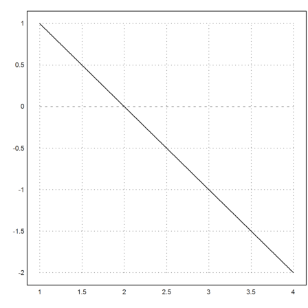
In this example, the derivative becomes positive for y between 0 and -c, where c is a very small number. The simple Runge algorithm simply overshoots this area, and effectively solves the equation y'=-1.
>c=1e-5; y=runge("-y/(c+y)",x,1); ...
 plot2d(x,y):
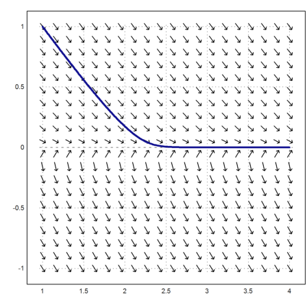
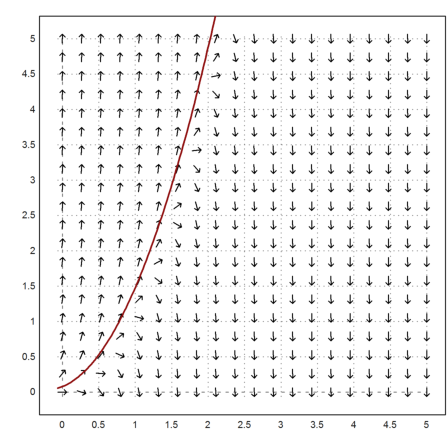
To make clear what is happening we plot the vectorfield for c=0.1. There is an area, where the derivative is large, but with very small c, the Runge method simply jumps over it.
>c=0.1; vectorfield("-y/(c+y)",1,4,-1,1); ...
 plot2d(x,runge("-y/(c+y)",x,1),add=1,color=blue,thickness=3); ...
 insimg;
This differential equation can be solved exactly with an implicit solution.
>&ode2('diff(y,x)=-y/(c+y),y,x)
- c log(y) - y = x + %c
We can plot this result as a function x=x(y).
>y=epsilon:0.01:1; x=-c*log(y)-y;  ...
 plot2d(x+2,y,a=1,b=4,c=-1,d=1,color=blue,thickness=3):
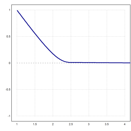
The adaptive Runge method, which is carefully adjusted to work for such problems, can solve the differential equation, but the adaptive steps are very small after the equation has become stiff.
So be prepared to wait a few seconds for the result.
>c=1e-5; x=1:0.1:4; y=adaptiverunge("-y/(c+y)",x,1); ...
 plot2d(x,y):
Euler has the LSODA solver, which can switch to a special mode for stiff equations. It works very well and should be the method of choice.
>c=1e-5; x=1:0.1:4; y=lsoda("-y/(c+y)",x,1,epsilon); ...
 plot2d(x,y):

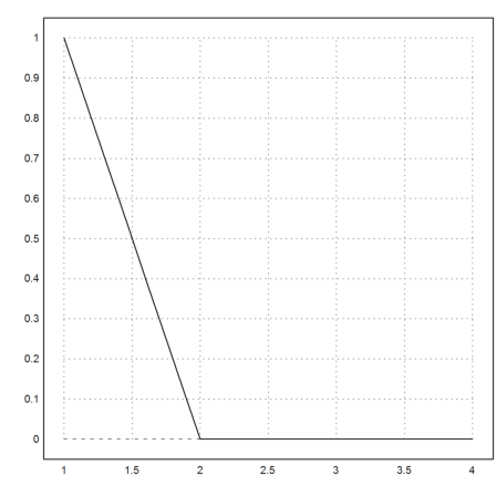
To overcome the stiffness, the differential equation could have been limited. This is pobably the intention anyway. The following works much faster, even for smaller c.
>c=1e-7; y=adaptiverunge("min(-y/(c+y),0)",x,1); ...
 plot2d(x,y):

Let us consider another example which is discussed in "Integration of Stiff Equations" by Curtiss and Hirschfelder.
![]()
>function f(x,y) := 5*(y-x^2)
The problem can be solved by Maxima.
>sol &= ode2('diff(y,x)=5*(y-x^2),y,x);
Let us define a function from the solution.
>function fsol(x,%c) &= expand(y with sol)
                           5 x    2   2 x   2
                       %c E    + x  + --- + --
                                       5    25
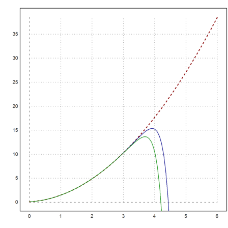
We can draw the vectorfield and add a specific solution. From the vector field it is obvious that the solution will not be stable.
>vectorfield("f",0,5,0,5); ...
 c=-20; plot2d("fsol(x,0)",add=1,color=red,thickness=2):
Let us plot this unstable solution, and add the results of the Runge and the adaptive Runge method. Both fork off the solution quite rapidly.
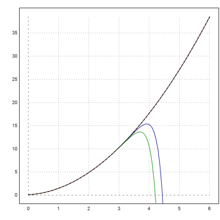
>plot2d("fsol(x,0)",0,6,color=red,thickness=2,style="--"); ...
 x=0:0.01:6; y=runge("f",x,2/25); ...
 plot2d(x,y,add=true,color=blue); ...
 plot2d(x,adaptiverunge("f",x,2/25),add=true,color=green):
And the lsoda method stays on track, showing its ability to select a particular solution even when faced with instabilities.
>plot2d(x,lsoda("f",x,2/25),add=true,color=black):
The following example was brought to my attention by Radovan Omorjan. I cite his notebook.
It is Problem No. 6.1 from: "M.B.Cutlip, M.Shacham, Problem Solving in Chemical and Biochemical Engineering ..., Second Edition, Prentice Hall (2008)"
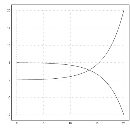
The biological process model of biomase (B) and substrate concentration (S) time dependence is given in the form of differential equations:
![]()
t=(0,20] given the initial conditions:
![]()
with the reaction kinetic parameters (k,K).
>k=0.3; K=1e-6;
>function dY (t,y) ...
   global k,K
   dBdt=k*y[1]*y[2]/(K+y[2]);
   dSdt=-0.75*k*y[1]*y[2]/(K+y[2]);
   return [dBdt,dSdt];
 endfunction
Set some initial conditions.
>B0=0.05; S0=5; y0=[B0,S0];
And the time interval.
>t0=0; tf=20; t=t0:0.1:tf;
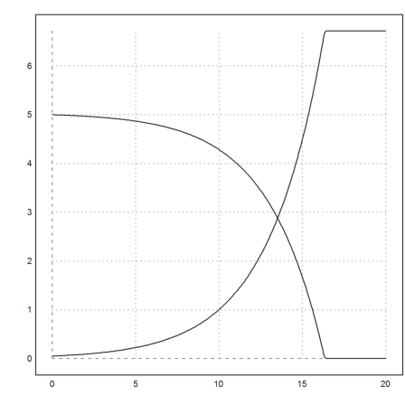
Now, try the Runge method. As above, the value for S will overshoot 0, and become negative. The solution is not correct from that point on.
>y=runge("dY",t,y0); ...
 plot2d(t,y):
Again, the LSODA algorithm works well.
>y=lsoda("dY",t,y0); ...
 plot2d(t,y):

The adaptive Runge method at the default accuracy would take very, very long.
It is more sensible to stop at a zero amount of substrat.
>function dY (t,y) ...
   global k,K
   dBdt=k*y[1]*y[2]/(K+y[2]);
   dSdt=min(-0.75*k*y[1]*y[2]/(K+y[2]),0);
   return [dBdt,dSdt];
 endfunction
Now, everything works as expected.
>y=adaptiverunge("dY",t,y0); ...
 plot2d(t,y):
To test the various algorithms, let us try the following example.
>function f(x,y) ...
 useglobal;
 itercount=itercount+1;
 return -2*x*y
 endfunction
The differential equation is simply
![]()
We integrate it from 0 to 5.
>x=0:0.01:5;
The correct result.
>exp(-25)
0
The Runge method delivers a very good result taking 2000 function evaluations.
>itercount=0; y=runge("f",x,1); itercount, y[-1],
2000
0
The adaptive method takes more function evaluations, and the result is not much better.
>itercount=0; y=adaptiverunge("f",[0,5],1); itercount, y[-1],
6775
0
The LSODA method used by ode takes only a few evaluations, but the result is not so good.
This is an example of a function, where the LSODA algorithm takes many steps, and needs to be reset at each step. In other words, it is not a good algorithm here.
>itercount=0; y=ode("f",0:0.001:5,1,reset=true); itercount, y[-1]
64784
0